Deep Learning Architectures

 Deep learning architectures, which have become more competitive with the ImageNet competition, which is a worldwide competition, are increasing more and more with the changing number of layers and success rates every year. It would not be wrong to say that the AlexNet architecture started this race. For this reason, the sample layer description below is made on the AlexNet architecture, and a general explanation is made for other architectures.

AlexNet: Deep convolutional neural network for image classification, winner of the ILSVRC-2012 competition. It consists of eight layers, the first five of which are convolutional and the last three are fully connected layers. Among these layers there are also “pooling” and “activation” layers. There are also input and output layers. The AlexNet architecture is designed to classify 1000 objects and the error rate in object identification has been reduced from 26.2% to 15.3%. The AlexNet architecture is shown in the figure [1].

AlexNet architecture

In the AlexNet diagram, it is seen that the problem is divided into two parts, with half running on GPU1 and the other half running on GPU2. Thus, the communication load is kept low, which helps to achieve a good overall performance. Data processing from the two channels is only crossed at the third feature extraction layer.

AlexNet layers a) 1st layer b) 2nd layer c) 6th layer

The first layer is the convolutional layer.

• Input image size: 224 x 224 x 3
• Number of filters: 96
• Filter size: 11 x 11 x 3
• Stride length: 4

Layer Output

• 224/4 x 224/4 x 96 = 55 x 55 x 96
• 55 x 55 x 48 per GPU when divided by 2 GPUs

The second layer is a Max Pooling layer followed by convolution.

• Input image size: 55 x 55 x 96
• Max Pooling: 55/2 x 55/2 x 96 = 27 x 27 x 96
• Number of filters: 256
• Filter size: 5 x 5 x 48

Layer Output

• 55/2 x 55/2 x 96 = 27 x 27 x 96
• 27 x 27 x 128 per GPU when divided by 2 GPUs

The third, fourth and fifth layers proceed similarly. The sixth layer is the fully bonded layer.

On the sixth layer, the input is transformed to a vector 13 x 13 x 128 and multiplied by 2048:

(13 x 13 x 128) x 2048

Here GEMV (General Matrix Vector Multiply) is used.

Vector X = 1 x (13x13x128)

Matrix A = (13x13x128) x 2048

Output: 1 x 2048

The seventh and eighth layers proceed similarly.

ZFNet: After AlexNet won the ImageNet competition, ZFNet [2], inspired by this architecture, became the winner of the ImageNet competition in 2013. With this architecture, the error rate in object recognition has been reduced to 11.2%. Difference from AlexNet; determines the filter size as 7x7 and the number of steps as two. Here, a smaller filter size in the first convolution layer is intended to help preserve a lot of original pixel information in the input size. In addition, it has used “Cross Entropy”, “Probabilistic Slope Descent” and “ReLU” algorithms in its architecture. ZFNet architecture consists of 7 layers. The figure shows ZFNet architecture.

ZFNet architecture

GoogLeNet: GoogleNet is a complex structure created from Inception modules and is the 2014 winner of the ImageNet competition. Unlike previous studies, the depth and width of the network prepared were increased while the calculation cost was kept low. Architecture consists of 22 layers. To optimize quality, architectural decisions are based on the Hebbian principle and the intuition of multi-scale processing. In the competition, he achieved a top-5 error rate of 6.67%. The GoogLeNet architecture is shown in the figure [3].

GoogLeNet architecture

RestNet: ResNet, which consists of 152 layers, has a deeper structure than previous architectures. It was the winner of the ImageNet competition in 2015 by achieving a 3.57% top-5 error rate. This rate exceeds the human error rate, meaning a great success. In the Residual blocks that make up the architecture, the x input produces an F (x) result after the convolution-ReLUconvolution series. This result is then added to the original entry x and expressed as H (x) = F (x) + x. An example ResNet architecture with 34 layers and Residual block structure is shown in Figure [4].

a) RestNet 34-layer architecture b) Residual block

VGG16 — VGG19: There are two different types of VGGNet architecture, 16 and 19 layers; VGG16, VGG19. The number of layers is determined by the number of weight layers. VGG16 architecture is an architecture that consists of 13 convolution 3 fully connected layers used to achieve better results in ImageNet 2014 competition [5]. There are 41 layers in total, including MaxPooling, FullyConnectedLayer, ReLULayer, DropOutLayer and SoftmaxLayer layers. The image to be included in the input layer is 224x224x3. The last layer is the classification layer [6].

The VGGNet architecture uses 3x3 filters on all its layers and overlaps Convolution-ReLU layers before pooling layer. As in other deep architectures, the height and width dimensions of the matrices from the input layer to the exit decrease while the depth value increases in VGG architecture. In 2014, it achieved a top-5 error rate of 7.3%. VGGNet architecture is shown in the figure [5].

VGGNet architecture

REFERENCES

[1] Krizhevsky, A., Sutskever, I., and Hinton, G. E. (2012). 25th International Conference on Neural Information Processing Systems. ImageNet Classification with Deep Convolutional, 1097–1105. Lake Tahoe, Nevada: NIPS’12 Proceedings.

[2] Zeiler, M. D., and Fergus, R. (2014). Visualizing and Understanding Convolutional Networks. Computer Vision — ECCV 2014, 818–833. doi: 10.1007/978–3–319–10590–1_53

[3] Szegedy, C., Liu, W., Jia, Y., Sermanet, P., Reed, S., Anguelov, D., and Rabinovich, A. (2015). 2015 IEEE Conference on Computer Vision and Pattern Recognition (CVPR). Going deeper with convolutions, 1–9. Boston, MA, USA: IEEE. doi:10.1109/CVPR.2015.7298594

[4] He, K., Zhang, X., Ren, S., and Sun, J. (2016). 2016 IEEE Conference on Computer Vision and Pattern Recognition (CVPR). Deep Residual Learning for Image Recognition,1–12. Las Vegas, NV, USA: IEEE. doi: 10.1109/CVPR.2016.90

[5] Simonyan, K., and Zisserman, A. (2014). Very Deep Convolutional Networks for Large-Scale Image Recognition. Web: https://arxiv.org/abs/1409.1556

[6] Doğan, F., ve Türkoğlu, İ. (2018). Derin Öğrenme Algoritmalarının Yaprak Sınıflandırma Başarımlarının Karşılaştırılması. Sakarya Universıty Journal Of Computer And Informatıon Scıences, 1, 10–21.

[7] Savaş, S. (2019), Karotis Arter Intima Media Kalınlığının Derin Öğrenme ile Sınıflandırılması, Gazi Üniversitesi Fen Bilimleri Enstitüsü Bilgisayar Mühendisliği Ana Bilim Dalı, Doktora Tezi, Ankara.

Deep Learning

 

The success achieved as a result of the classification made by Krizhevsky and his friends through Deep Convolutional Neural Netrowks named AlexNet [1] in the competition to recognize the world’s most important objects named ImageNet in 2012 has been the greatest impact of deep learning in the world literature. After this success, deep learning has been on the rise. Deep learning was first introduced in the literature in 2006 with a method called deep thought networks [2]. Deep Belief Nets (DBN) were tested using the preferred MNIST (image data of 70,000 28 x 28 pixel handwritten characters ranging from 0–9) to measure and estimate the accuracy of each image recognition method. The development of deep learning over time is shown in Figure [3].

In recent years, techniques developed in deep learning research affect a wide range of information processing studies in expanded scopes, in both traditional and new forms, including the most effective and important aspects of machine learning and artificial intelligence.

Although deep learning is a sub-field of machine learning, it is the application area of deep neural networks that is becoming widespread day by day. Instead of specialized algorithms for each study in this field, it is aimed that solutions based on learning data cover a wider data set. Deep learning is a promising approach to solving artificial intelligence problems in machine learning.

There are various definitions of deep learning [4]:

Definition 1: A class of machine learning techniques that uses multiple nonlinear computing layers for supervised or unsupervised feature extraction and transformation, model analysis, and classification.

Definition 2: A subfield within machine learning that relies on algorithms to learn multiple levels of representation to model complex relationships between data. Thus, high-level features and concepts are defined as low-level features, and such a hierarchy of features is called a deep architecture. Most of these models are based on learning from unsupervised representations.

Definition 3: It is a subfield of machine learning based on the learning of several levels of representation that correspond to a hierarchy of features or factors or concepts in which higher-level concepts are defined from lower-level concepts, and the same low-level concepts can help define many higher-level concepts. Deep learning is part of a wider family of machine learning methods based on learning representations. An observation (e.g., an image) can be represented in many ways (e.g., a pixel vector), but some displays make it easier to learn interesting tasks (e.g. is this the image of a human face?) From examples and research in this field, what is better? It tries to determine how it can be represented and how to learn.

Definition 4: Deep learning is a set of algorithms trying to learn at multiple levels corresponding to different levels of abstraction in machine learning. Artificial neural networks are generally used. In these learned statistical models, the levels correspond to different concept levels where higher-level concepts are defined from lower-level concepts, and the same low-level concepts can help define higher-level concepts.

Definition 5: Deep Learning is a new area of machine learning research that has been introduced with the aim of bringing machine learning closer to one of its original purposes (artificial intelligence) Deep learning is about learning multiple levels of representation and abstraction that help in understanding data like images, sounds, and texts.

Deep learning is a machine learning technique that uses the deep neural network. Deep neural networks are multi-layered neural networks containing two or more hidden layers [5].

In deep learning, there is a structure based on learning more than one feature level or representation of data. High-level features create a hierarchical representation derived from lower-level features [6]. The representation for an image can be a vector of density per pixel values or features such as edge clusters, custom shapes. Some of these features represent the data better. In deep learning methods, effective algorithms are used for hierarchical feature extraction that best represents the data, instead of the manually extracted features [7].

There are two main aspects common to the various high-level definitions of deep learning [4]:

• Models consisting of multiple layers or nonlinear computing stages,
• Methods for the supervised or unsupervised learning of feature representation in successive higher, more abstract layers.

High capacity (especially GPU) machines and large amounts of data are needed to run deep learning algorithms and solve problems. Unlike standard machine learning algorithms that break down problems and solve them individually, deep learning solves the problem from start to finish. More importantly, the more data a deep learning algorithm is fed, the better the task execution. Also, the time factor is important. Not time-bound studies can produce better results when fed with big data.

Three major reasons for the popularity of deep learning today are greatly increased processor capabilities (e.g., graphics processors (GPU)), massive increase in data used for education, and recent advances in machine learning and signal / information processing research. These developments have enabled deep learning methods to effectively utilize complex, compound nonlinear functions, learn distributed and hierarchical feature representations, and effectively use both labeled and unlabeled data [4].

In machine learning, the algorithm distinguishes between a square and a triangle based on information provided by humans. In deep learning, the program does not start with pre-fed information. Instead, it uses an algorithm to determine how many corners the shapes have, whether those corners are connected, and whether they are perpendicular. The algorithm ultimately determines whether an added circle fits the order of squares and triangles.

Solving problems such as image and / or sound identification, which can be easily done by humans, is difficult for artificial intelligence methods. These intuitive problems can be solved by computers learning the ability of the simplest concepts to understand and experience the world hierarchically. With the knowledge gained through experience, there is no need for formulas and calculations specific to each problem used by computers. When the hierarchical structure is considered as a graphic, a deep multi-layered structure is formed, each of which is built on top of the other. For this reason, artificial intelligence methods based on hierarchical structure emerge as deep learning [8].

The research areas of deep learning neural networks are at the intersection between artificial intelligence, graphic modeling, optimization, pattern recognition and signal processing [4]. These algorithms have started to show themselves in many applications such as driverless vehicles, health services, movie suggestions, translation services, chatbots, page suggestions, advertising services.

The factors that make deep learning architectures such a popular field of study are as follows:

• Making common text, image and sound datasets available for research around the world.
• The production of high processing power graphics cards (GPU).
• AlexNet, ZFNet, ResNet, GoogLeNet, VGG16–19, Inception etc. The introduction of deep architectures such as.
• Keras, Tensorflow, Theano, Caffe, Pytorch, MatConvNet etc. The use of deep learning platforms and libraries such as.
• Activation functions, data training and data augmentation methods and effective optimizers are developed and put into use by researchers.

Deep neural networks have two or more hidden neural network layers. In deep neural networks, more comprehensive relationships are established from simple to complex in data. Each layer tries to establish a relationship between the previous layer and itself. Thus, a more detailed examination is made about the inputs and a more accurate decision is made. The figure shows a deep neural network structure with three hidden layers.

Deep neural network structure

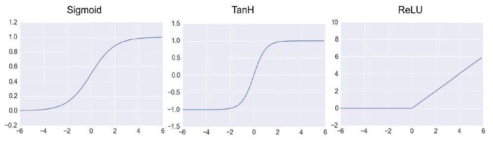
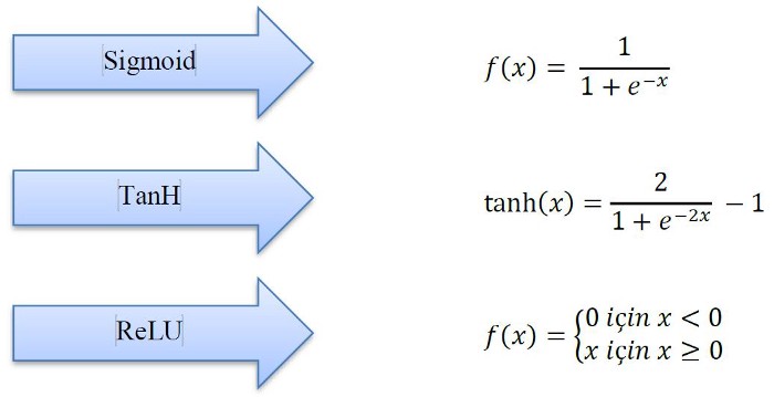
Different activation functions can be used while building deep neural networks. These functions can vary according to the type, structure, size of the data and the person creating the model. The activation function determines the output this cell will produce in response to the input to the cell. Usually a nonlinear function is chosen. Major activation functions are Sigmoid, TanH and ReLU.

Activation functions

Activation functions formulas

REFERENCES

[1] Krizhevsky, A., Sutskever, I., and Hinton, G. E. (2012). 25th International Conference on Neural Information Processing Systems. ImageNet Classification with Deep Convolutional, 1097–1105. Lake Tahoe, Nevada: NIPS’12 Proceedings.

[2] Hinton, G. E., Osindero, S., and Teh, Y.-W. (2006). A fast learning algorithm for deep belief nets. Neural Comput, 1527–1554.

[3] Ay Karakuş, B. (2018). Derin Öğrenme ve Büyük Veri Yaklaşımları ile Metin Analizi. Doktora Tezi, Fırat Üniversitesi Fen Bilimleri Enstitüsü, Elazığ.

[4] Deng, L., and Yu, D. (2013). Deep Learning Methods and Applications. Foundations and Trends in Signal Processing, 7, 197–387. doi: 10.1561/2000000039

[5] Phil, K. (2017). MATLAB Deep Learning: With Machine Learning, Neural Networks andArtificial Intelligence. Seoul, Soul-t’ukpyolsi, Korea: Apress.

[6] Bengio, Y. (2009). Learning Deep Architectures for AI. Foundations and Trends in Machine Learning, 2, 1–127. doi: 10.1561/2200000006

[7] Song, H. A., and Lee, S.Y. (2013). International Conference on Neural Information Processing. Hierarchical Representation Using NMF, 466–473. Daegu, South Korea.

[8] Goodfellow, I., Bengio, Y., and Courville, A. (2016). Deep Learning. MIT Press. http://www.deeplearningbook.org

[9] Savaş, S. (2019), Karotis Arter Intima Media Kalınlığının Derin Öğrenme ile Sınıflandırılması, Gazi Üniversitesi Fen Bilimleri Enstitüsü Bilgisayar Mühendisliği Ana Bilim Dalı, Doktora Tezi, Ankara.

Limitations of Machine Learning

 

Along with the opportunities and benefits that machine learning systems provide, there are also limitations and challenges. These limitations can be explained as follows:

Determining the appropriate algorithm for the learning problem is one of the most important problems for machine learning. Researchers need to be able to determine the algorithm for the needs of the problem and test many different algorithms for this. Along with the algorithm, model parameters should also be determined. While some algorithms perform well for text processing, different algorithms for image processing may perform better.

The noise contained in the available data is another limitation of machine learning. The presence of structured and / or unstructured data at the same time between data heaps, which arise especially with the concept of big data, is another problem to be tackled in machine learning. Noise in data; Differences in the characteristics of an image such as size, color, resolution can appear in different ways such as misspellings, punctuation marks, special symbols and abbreviations used in a text data.

Feature extraction is one of the most important steps of the machine learning system as it changes depending on the correct operation of the system and the selection of the correct features and number of features. The feature extraction process depends on the problem with which the transaction is performed and is specific. To be more precise, the characteristics determined in a health problem will be different from the features that will be used for an autonomous vehicle. The extraction of a common feature produced for different problem solutions in different disciplines may benefit very large problem solutions in the future.

Over learning is another machine learning limitation. While the model created shows high performance during training, it may underperform or underperform than expected on test data. In this case, it is thought that the training data are memorized by the model, in other words, the model is over-learned. To prevent this, the complexity of the model is increased during the training and various methods are tried.

In controlled machine learning methods, the model is trained on the labeled data and the detection and diagnosis are performed. In order to construct this model, a considerable amount of large data should be available. For such a data labeling job, experts and hard work are required. It is also possible to cause human-induced errors. There may also be a lack of expert personnel in solving special problems. All of these come together to reveal the limitation of data labeling.

REFERENCE

Savaş, S. (2019), Karotis Arter Intima Media Kalınlığının Derin Öğrenme ile Sınıflandırılması, Gazi Üniversitesi Fen Bilimleri Enstitüsü Bilgisayar Mühendisliği Ana Bilim Dalı, Doktora Tezi, Ankara.

Reinforcement Learning

 In this learning, the answer to the question of how an autonomous agent perceiving and acting in his / her environment can learn to do the most appropriate actions to achieve his goal [1]. It is widely used in systems such as robotics, game programming, disease diagnosis and diagnosis, automation.

In response to an act of the agent in the reinforced learning environment, the trainer or software reinforces the agent with a reward or punishment to indicate the status of the new situation. Thus, in this system, the best action that can be taken to achieve the goal tries to be selected [2].

There are two main methods for solving problems with reinforcement learning: The first is to search the training space to find the one that improves the environment, and the second is to use statistics and dynamic programming methods to predict useful motion [3].

The purpose of reinforcement learning is to find the optimal policy. Optimal policy enables the agent to optimally solve the problem and reach the result. Thus, the agent reaches its target highest reward value. The optimal policy can be expressed as the maximum value of the reduced total reward amount starting from a random st state. The goals and awards determined by the instructor or the software are of great importance in order to achieve the goal of reinforcement learning. For this reason, it is seen that purpose and rewarding affect the success and how important it is in systems designed with reinforced learning method [4].

The most obvious difference of reinforced learning from supervised learning is that only some feedback is given to the agent for the predictions of the agent. In addition, the predictions here can have a long-term effect on the future state of the controlled system. Thus, time becomes an important factor [5].

In a reinforced learning system, there are four elements, one optional, besides the factor and the environment [6]:

• policy
• reward signal
• value function
• model

Policy; It determines the action the agent can take in the situation he is in. Prize; It is the score received from the environment for an action performed by the agent. Status value; It is the sum of the rewards that the agent can expect from the situation and other situations that follow that situation. Model; It is an element that is optionally included in the system [6].

Temporal difference learning (TD learning): Before explaining temporal difference learning, it is necessary to start with a basic understanding of value functions. Value functions are state-action pair functions that predict how well a particular action will do in a given situation, or predict what the return of that action will be. Value functions representation [7]:

Vπ (s) — value of state s in policy π.
Qπ (s, a) — the value (Q value) of state s in policy π to perform move a.

The problem here is to estimate these value functions for a particular policy. The reason for predicting these value functions is that they can be used to accurately select an operation that will provide the best possible total reward once it occurs in a given situation [7].

The TD learning method is a reinforced learning algorithm that can learn directly from raw experiences without the dynamics of the environment model. In this method, predictions based on other learned predictions are partially updated (booted) without waiting for a final result [3]. In the TD learning method, predictions are used as a goal in the learning process. As a model-free learning algorithm, TD learning has two important features:

• It does not require prior knowledge of model dynamics.
• It can also be applied for non-episodic tasks.

TD can be used to predict learning value functions. If the value functions were to be calculated without predicting, it would be necessary to wait for the final reward before any state-action pair values were updated. Once the final reward has been received, the path taken to reach the final state would have to be taken back and each value updated accordingly. Instead, with TD learning methods, an estimate of the final reward in each case is calculated and the state-action value is updated for each step of the situation.

The TD learning method is called the “bootstrap” method because the value is partially updated using an existing estimate, not a final reward. TD learning can be organized in two ways as “Political” and “Non-Policy” Learning. Methods in policy learning learn the value of the policy used to make decisions. Value functions are updated using the results of performing actions specified by some policies. These policies are usually soft (always assuring politics an exploratory element) and not deterministic. The policy is not strict and always chooses the action that gives the most reward. There are three types of frequently used policies: soft, greedy and softmax. Non-policy methods can learn different policies for behavior and prediction. The policy of conduct is usually lenient. Non-policy algorithms can update predictive value functions using hypothetical actions that were actually untested. Non-policy algorithms can separate research from control and intra-policy algorithms cannot. An agent trained using a non-policy method may result in learning tactics that should not necessarily be demonstrated during the learning phase.

Q learning: It is one of the most commonly used reinforcement learning algorithms. Q learning is an algorithm that can learn online in environments where there is no information about the environment. In a random environment, the agent is shown how to learn the optimal policy. It is difficult for the agent to learn the optimal policy directly. Because there is no training data that can be used for your agent. The training data available to the agent are only instant rewards. It is easier to learn a numerical evaluation function using these training data and then determine the optimal policy with the help of this function [4].

TD is a non-policy algorithm for learning. The main purpose of the Q learning algorithm is to examine the next moves and see the reward it will gain according to the moves it will make, and to act in a way that will maximize this award. In this algorithm, the agent is expected to set up a plan for the future. This algorithm is often applied to problems such as maze and search.

The algorithm is basically based on two matrices. The first matrix is the Reward matrix, the other is the State matrix. Moving during a given repetition, the robot completes the S matrix through the values in the R matrix during these movements. The last values of the S matrix formed as a result of all repetitions show the optimal result.

Q learning is a model-independent Reinforcement Learning algorithm that can be easily applied to areas that can be modeled as the finite state Markov Decision Process. Reinforcement learning problems can be modeled mathematically like Markov decision processes. Markov decision process is defined based on the following parameters [8].

• The finite set of states, S
• Set of movements, A
• A reward function, R: S x A → R
• State transition function, T: S x A → π (S)

Here π (S) can be defined as a probability distribution over the set S. The state transition function determines possibly the next state of the environment as a function of the current state and motion of the agent. The reward function gives instant rewards. This feature is known as the Markov Feature. Accordingly, there is no dependence between the past state, action, and reinforcement. Therefore, Markov decision process defines the dynamics of the environment for only one step [8].

The Q learning procedure can be listed as follows:

• Start the table of Q-values (Q (s, a)).
• Observe the current situation, p.
• Choose an action based on one of the action choice policies. (soft, greedy or softmax).
• Take action and watch the reward (r) and new status (s’).
• Update the Q value for the status using the reward observed and the maximum possible reward for the next situation.
• Set the state to its new state and repeat the process until you reach the terminal state.

SARSA: The Sarsa algorithm is a policy algorithm for TD learning. The biggest difference between Sarsa and Q learning is that the maximum reward for the next state is not necessarily used to update the Q values. Instead, a new action, and hence the reward, is selected using the policy that determines the original action. In the current state, S is taken an action, “A” and the agent gets a reward, “R” and ends in the next case, “S1” and takes action, A1 on S1. Based on this, it was named (S, A, R, S1, A1).

The SARSA procedure can be listed as follows:

• First, reset the Q values to some arbitrary value,
• Choose an action according to Epsilon-greedy policy and move from one state to another,
• Update Q value in previous state, following update rule.

REFERENCES

[1] Kaelbling, L. P., Littman, M. L., and Moore, A. P. (1996). Reinforcement learning: A Survey. Journal of Artificial Intelligence Research, 237–285.

[2] Hoshino, Y., and Kamei, K. (2003). SICE 2003 Annual Conference. A proposal of reinforcement learning system to use knowledge effectively, 1582–1585. IEEE Xplore.

[3] Sutton, R. S., and Barto, A. G. (1998). Reinforcement Learning: An Introduction. Cambridge: MIT Press.

[4] Hacıbeyoğlu, M. (2006). Çoklu Etmen Mimarisi ve Takviyeli Öğrenme. Bilgisayar Mühendisliği Anabilim Dalı, Yüksek Lisans Tezi, Selçuk Üniversitesi Fen Bilimleri Enstitüsü, Konya.

[5] Szepesvari, C. (2010). Algorithms for Reinforcement Learning. Morgan & Claypool. doi: 10.2200/S00268ED1V01Y201005AIM009

[6] Kayaoğlu, T., Bilgiç, T., Özkaynak, S., Çalışır, S., ve Güçkiran, K. (2018). Pekiştirmeli Öğrenmeye Giriş Serisi-1. Web: https://medium.com/deep-learningturkiye/peki%CC%87%C5%9Fti%CC%87rmeli%CC%87-%C3%B6%C4%9Frenmeye-gi%CC%87ri%CC%87%C5%9Fseri%CC%87si%CC%87-1-8f5c35b6044

[7] Eden, T., Knittel, A., and Uffelen, R. v. (2019). Reinforcement Learning. Web: http://www.cse.unsw.edu.au/~cs9417ml/RL1/tdlearning.html

[8] Kaya, M. (2003). Çoklu Etmen Takviyeli Öğrenmeye Veri Madenciliği Tabanlı Yeni Yaklaşımlar, Doktora Tezi, Fırat Üniversitesi Fen Bilimleri Enstitüsü. Elazığ.

[9] Savaş, S. (2019), Karotis Arter Intima Media Kalınlığının Derin Öğrenme ile Sınıflandırılması, Gazi Üniversitesi Fen Bilimleri Enstitüsü Bilgisayar Mühendisliği Ana Bilim Dalı, Doktora Tezi, Ankara.